jgkilian777.github.io
Project maintained by jgkilian777 Hosted on GitHub Pages — Theme by mattgraham
Disclaimer: this is an attempt to summarise over 400 pages of documentation and the intention is more to display rather than fully explain the methods developed.
This was a personal project focussing on developing a puzzle solving methodology that fully prioritised implementation speed over readability and good coding practices. There are debugging remnants, bad code structure, code duplication, unuseful object naming and (very rarely) inefficient code.
The entire project that contained a total of over 40,000 lines of code was regrettably written using notepad++.
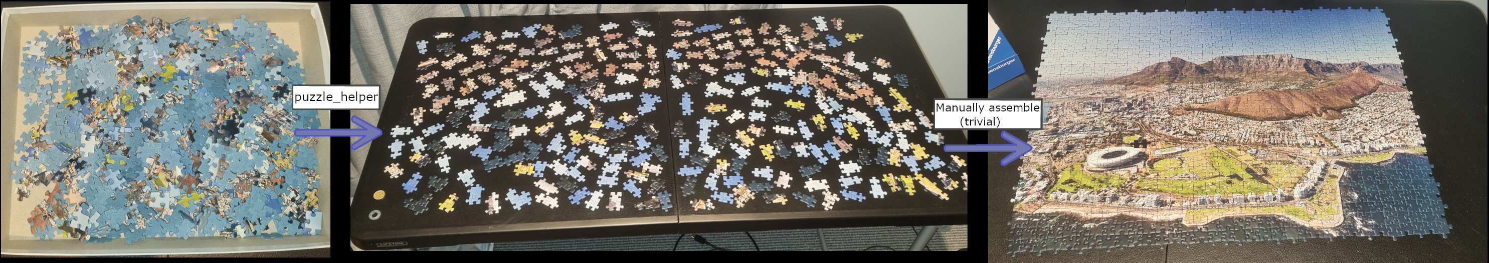
Key outcomes/results:
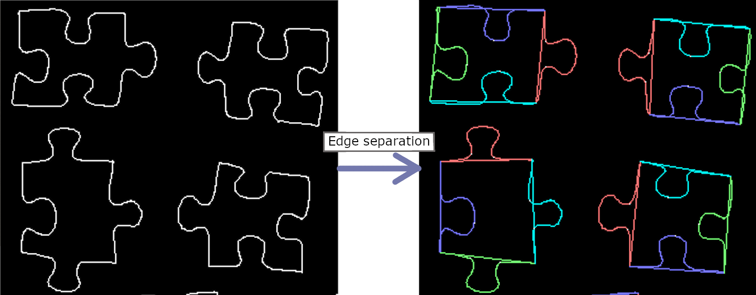
Robust method for splitting jigsaw pieces into distinct edges
 Uses amount of defects paired with information about the areas at the start and end of each defect’s hull (whether the hull starts/ends at a turning point or a roughly flat area, and how close 2 consecutive defects’ hulls are to each other)
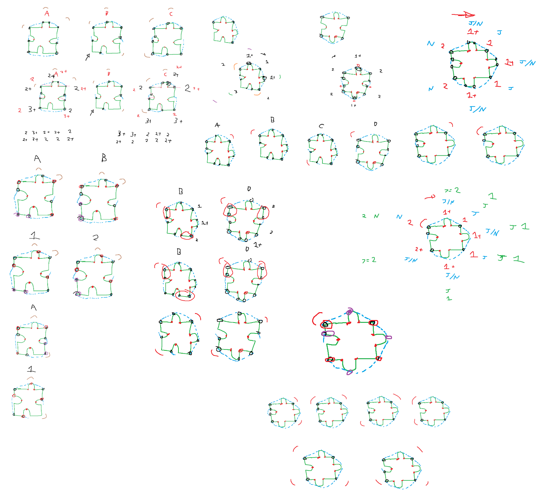
Example case: 7 Defects. All pairs of defects potentially form a nub except 2 pairs.
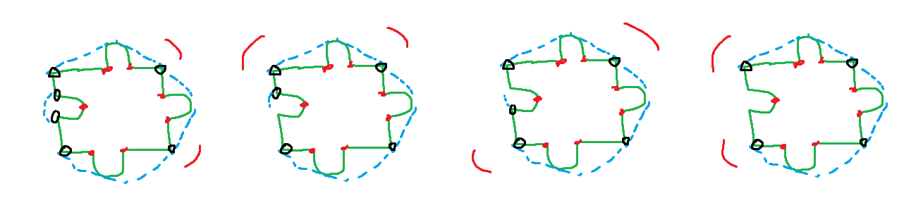 We have 2 pairs of defects that we know do not surround a nub.
If the 2 pairs share a defect, it is the 4th diagram with the shared defect being inside the innie. In this case the corners can easily be found because the defect pairs that each surround a nub are known, so the corners are simply a combination of the start/end points of the hulls of the first/second defects surrounding the nubs.
If the 2 pairs are not directly next to eachother, then it is the 3rd diagram (there are 1+ defects between the 2 pairs). Again, given this known schema, it is easy to retrieve the corners.
We have 2 pairs of defects that we know do not surround a nub.
If the 2 pairs share a defect, it is the 4th diagram with the shared defect being inside the innie. In this case the corners can easily be found because the defect pairs that each surround a nub are known, so the corners are simply a combination of the start/end points of the hulls of the first/second defects surrounding the nubs.
If the 2 pairs are not directly next to eachother, then it is the 3rd diagram (there are 1+ defects between the 2 pairs). Again, given this known schema, it is easy to retrieve the corners.
If it is neither of the above scenarios, then we have either the first or second diagram. If both pairs of defects have hulls that join in the middle, it is the first diagram, as they join on the corners (the second diagram has 1 pair joining in the middle at a corner, and 1 pair not joining). Since we know the schema based on the information about the middle joins, it is easy to retrieve the corners in either case.
The code for all cases can be found from here until the end of the function around 2300 lines after.
Compatibility
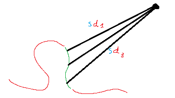
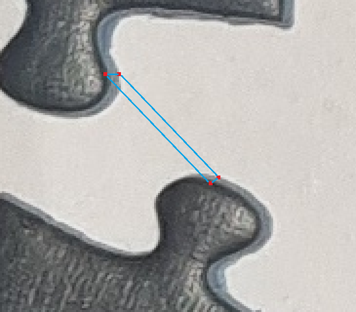
Edge1 and Edge2 are compatible if:
- Edgespans (red line) have similar lengths after accounting for scale (with error)
- Respective wingspans have similar lengths (blue lines, wings are defined by lines from the nub defects outwards)
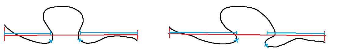
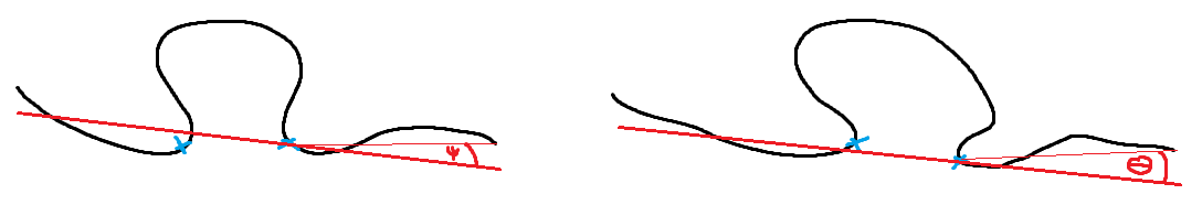
- The respective wing angles are similar enough (a wing angle is defined by the angle difference between the orientation of the wing and orientation of the full edgespan)
- The colours in a neighbourhood from the edge are similar enough, e.g. within a threshold difference calculated using CMC l:c difference measure in L*C*h colour space.
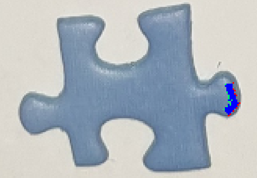
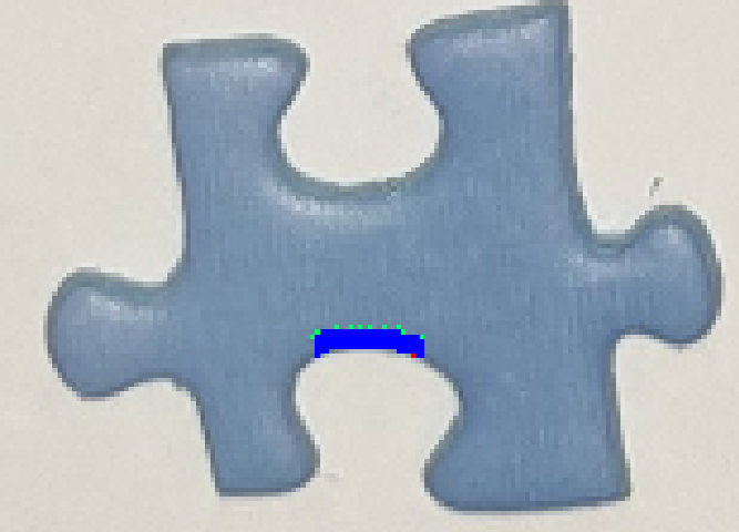
Colour Compatibility
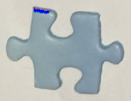
I split the edge into equal arclength segments (red points below), then calculate points at a given distance inwards (green points below) which gives a polygon, then I get the average colour in the polygon and store it.Note: in the first 2 images below, the polygon has been shifted inwards and in the 3rd image the red points in the polygon start right at the edge of the piece. This is because in the first 2 images, the blue cardboard material that the pieces are made with is showing because of the way the piece is orientated with respect to the camera, and we don’t want that colour to be part of the average colour so I first check if it’s possible for the camera to see the piece material (based on edge orientation w.r.t. center of the image) and if it is possible, I shift the red points inwards until the colour difference between the neighbourhood and the piece material is large enough to be considered different.
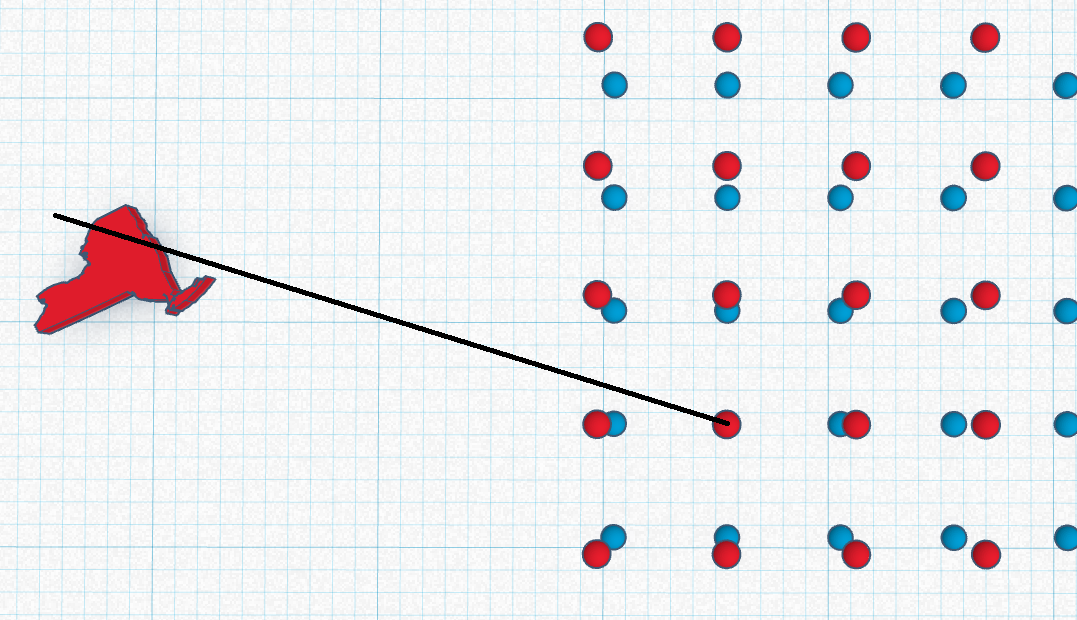
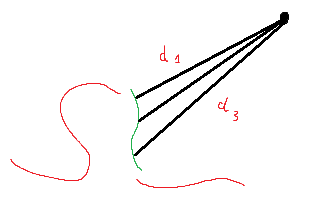
Using the line between the orthogonal projection of camera world coordinates onto the table plane and points on the jigsaw pieces
I noticed that, given 2 parallel planes, and an image taken s.t. the image plane is parallel to the 2 planes, if the line drawn from the center of the image intersects with a point from one of the parallel planes, then it also intersects with the respective point in the other plane. If the image plane isn’t parallel to both of the parallel planes, then this still holds true but the line will be drawn from the point that is the orthogonal projection of the camera position in world coordinates onto the parallel planes rather than the point at the center of the image.
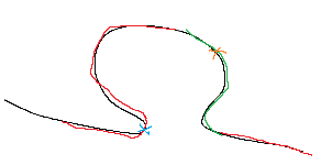
Below shows the line from this point being collinear with the line segment between a pointPair of the 2 parallel planes (2 points at the green arrows, this line segment is also obviously orthogonal to both planes).
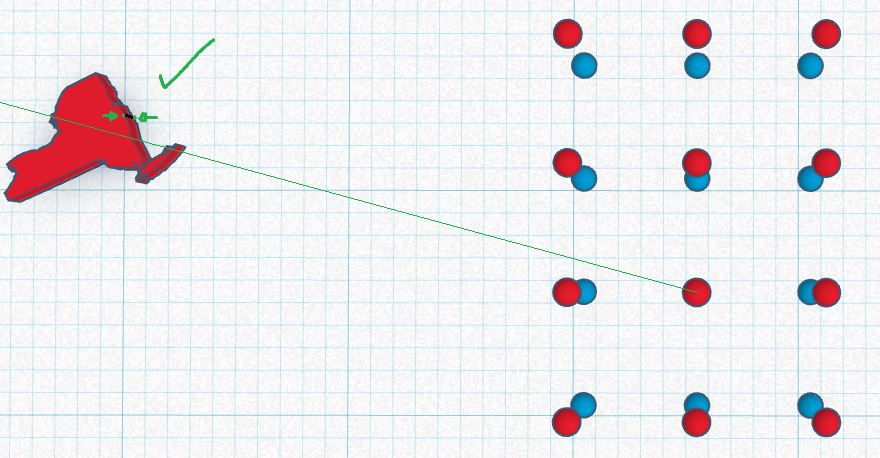
Using this center image point and the direction of the tangent at each point of each edge, we can split edges into points that are on the bottom plane, and points that are on the top plane. This plane issue is caused by the piece material being visible because of their position on the table w.r.t. the camera. Since jigsaw pieces are right prisms, the full edge on the bottom plane is exactly the same as the full edge on the top plane, but only parts of either plane are visible from a photograph so we just need to split them accurately then try and find ways to align/match segmented edge data of one edge to segmented edge data of another edge.
Below is an example of using the direction of the edge (black arrow) w.r.t. the line from the center image point, to accurately split the edge into the top plane (blue) and the bottom plane given by visibility of the piece material (red).
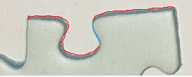
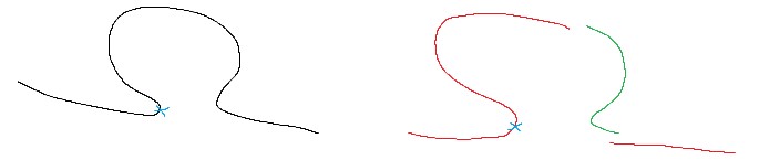
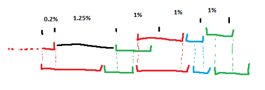
It’s also known that the edge segments in one plane can be shifted to the other plane from the center image point by a scale factor s.
Below is a simple example where the black edge1 fully appears on a single plane, and the second edge2 has been segmented into parts that appear on separate planes in red and green.
One of the nub defects is denoted by a blue x and it’s assumed that if these 2 edges match, then these defects at least roughly correspond.
First translate the edges so that the blue x defects are at the same point.
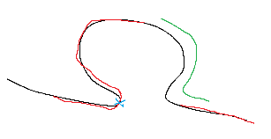
Since the defect appears in the red plane in edge2, I assume the red plane is now aligned with the single plane for edge1.
Then draw a line from the center image point in edge2 space to a point in the green plane of edge2 and find its respective point in edge1 space (which is now also edge2 red plane space), this will be the intersection between the line and the black plane in edge1.
Then scale the green plane to align this pointPair.
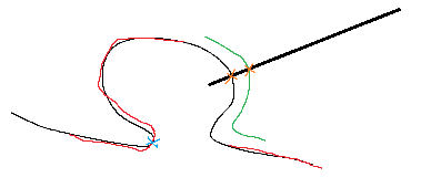
(It’s a bit more complicated than described, especially when both edges are separated into 2 planes)
I threw together an android app to help me keep the phone/camera parallel to the plane that the pieces were on. The 2 triangles are congruent when the phone is perfectly parallel and the angle difference between current phone orientation and parallel orientation is calculated using initial calibration values of the accelerometer and the current values. The gyroscope was too inaccurate for this purpose.
Icp
A variation of the iterative closest point algorithm is used with the transformation estimation step utilizing the closed-form solution for similarity transformation parameters by Shamsul A. Shamsudin and Andrew P. Murray.
There are many cases at this stage depending on the initial results of performing ICP on the 4 combinations of choosing 1 of the 2 planes from edge1 and 1 of the 2 planes from edge2. For example if the initial ICP executions result in plane1 from edge1 being fully paired to points in plane2 from edge2, and plane2 from edge1 being fully paired to points in plane1 from edge2, this would most likely mean both edges swap between planes at the exact same places, a simple case that would probably end there.
Other methods
Polyline convex hull implementation
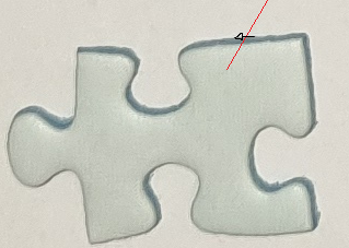
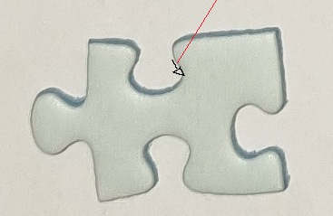
OpenCV convexHull had a bug that caused it to fail when given a self-intersecting contour so I implemented a modified version of Melkman's convex hull algorithm for polylines to properly handle any possible edge or piece data in this project. I also had to implement a convexity defects function that can robustly handle cases where there is 1 convex hull with 2 distinct convexity defects with a local maximum separating them like in the piece shown here:
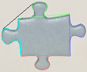
(The black line defines a convex hull but we actually want 2 defect points as if the single hull were split into 2 hulls at the corner point)
First edge matching attempt + solution for real world aspect ratio of a rectangle given image coords of its corners and its use in correcting perspective distortion in theory
The first edge matching implementation was simply uniformly sampling each edge, roughly aligning them using basic features and finding the distance between the 2 sets of edge points. This only works when there’s no difference in scale between any 2 edges and when given an orthographic view of the pieces where none of the bottom plane or piece material is visible, which is never the case.
I decided to try and find ways to normalise the data so it could be compared easily rather than creating a new comparison method that can handle data with scale/plane visibility differences. My intuition told me that there were almost certainly enough known variables to normalise a single image of 2 parallel planes (up to scale) given only 2 pairs of corresponding points and without using extra data such as intrinsic/extrinsic camera parameters. I knew that, if it were possible, it probably wouldn’t actually be useful in this context because it would be highly sensitive to noise but I was interested in finding out more and there is essentially no research available online for this specific problem so I spent a few weeks working on it to get the answer:
Given image coordinates for the 4 corners of a rectangle (y11, y12) (y21, y22) (y31, y32) (y41, y42), the real world aspect ratio of the rectangle is given by the formula below:
sqrt((-1 + (y11*y42*y22 - y11*y32*y22 + y31*y12*y22 - y31*y42*y22 - y12*y41*y22 + y41*y32*y22)/(y22*(y21*y42 - y21*y32 - y31*y42 + y31*y22 + y41*y32 - y41*y22)))**2*(-y11**2*y32*y22 + y11*y21*y32*(y11*y42*y22 - y11*y32*y22 + y31*y12*y22 - y31*y42*y22 - y12*y41*y22 + y41*y32*y22)/(y21*y42 - y21*y32 - y31*y42 + y31*y22 + y41*y32 - y41*y22) + y11*y31*y22*(-y11*y42*y32 + y11*y32*y22 - y21*y12*y32 + y21*y42*y32 + y12*y41*y32 - y41*y32*y22)/(y21*y42 - y21*y32 - y31*y42 + y31*y22 + y41*y32 - y41*y22) - y21*y31*(-y11*y42*y32 + y11*y32*y22 - y21*y12*y32 + y21*y42*y32 + y12*y41*y32 - y41*y32*y22)*(y11*y42*y22 - y11*y32*y22 + y31*y12*y22 - y31*y42*y22 - y12*y41*y22 + y41*y32*y22)/(y21*y42 - y21*y32 - y31*y42 + y31*y22 + y41*y32 - y41*y22)**2 - y12**2*y32*y22 + y12*y32*y22*(-y11*y42*y32 + y11*y32*y22 - y21*y12*y32 + y21*y42*y32 + y12*y41*y32 - y41*y32*y22)/(y21*y42 - y21*y32 - y31*y42 + y31*y22 + y41*y32 - y41*y22) + y12*y32*y22*(y11*y42*y22 - y11*y32*y22 + y31*y12*y22 - y31*y42*y22 - y12*y41*y22 + y41*y32*y22)/(y21*y42 - y21*y32 - y31*y42 + y31*y22 + y41*y32 - y41*y22) - y32*y22*(-y11*y42*y32 + y11*y32*y22 - y21*y12*y32 + y21*y42*y32 + y12*y41*y32 - y41*y32*y22)*(y11*y42*y22 - y11*y32*y22 + y31*y12*y22 - y31*y42*y22 - y12*y41*y22 + y41*y32*y22)/(y21*y42 - y21*y32 - y31*y42 + y31*y22 + y41*y32 - y41*y22)**2)/(y32*y22 - y32*(y11*y42*y22 - y11*y32*y22 + y31*y12*y22 - y31*y42*y22 - y12*y41*y22 + y41*y32*y22)/(y21*y42 - y21*y32 - y31*y42 + y31*y22 + y41*y32 - y41*y22) - y22*(-y11*y42*y32 + y11*y32*y22 - y21*y12*y32 + y21*y42*y32 + y12*y41*y32 - y41*y32*y22)/(y21*y42 - y21*y32 - y31*y42 + y31*y22 + y41*y32 - y41*y22) + (-y11*y42*y32 + y11*y32*y22 - y21*y12*y32 + y21*y42*y32 + y12*y41*y32 - y41*y32*y22)*(y11*y42*y22 - y11*y32*y22 + y31*y12*y22 - y31*y42*y22 - y12*y41*y22 + y41*y32*y22)/(y21*y42 - y21*y32 - y31*y42 + y31*y22 + y41*y32 - y41*y22)**2) + (-y11 + y21*(y11*y42*y22 - y11*y32*y22 + y31*y12*y22 - y31*y42*y22 - y12*y41*y22 + y41*y32*y22)/(y22*(y21*y42 - y21*y32 - y31*y42 + y31*y22 + y41*y32 - y41*y22)))**2 + (-y12 + (y11*y42*y22 - y11*y32*y22 + y31*y12*y22 - y31*y42*y22 - y12*y41*y22 + y41*y32*y22)/(y21*y42 - y21*y32 - y31*y42 + y31*y22 + y41*y32 - y41*y22))**2)/sqrt((-1 + (-y11*y42*y32 + y11*y32*y22 - y21*y12*y32 + y21*y42*y32 + y12*y41*y32 - y41*y32*y22)/(y32*(y21*y42 - y21*y32 - y31*y42 + y31*y22 + y41*y32 - y41*y22)))**2*(-y11**2*y32*y22 + y11*y21*y32*(y11*y42*y22 - y11*y32*y22 + y31*y12*y22 - y31*y42*y22 - y12*y41*y22 + y41*y32*y22)/(y21*y42 - y21*y32 - y31*y42 + y31*y22 + y41*y32 - y41*y22) + y11*y31*y22*(-y11*y42*y32 + y11*y32*y22 - y21*y12*y32 + y21*y42*y32 + y12*y41*y32 - y41*y32*y22)/(y21*y42 - y21*y32 - y31*y42 + y31*y22 + y41*y32 - y41*y22) - y21*y31*(-y11*y42*y32 + y11*y32*y22 - y21*y12*y32 + y21*y42*y32 + y12*y41*y32 - y41*y32*y22)*(y11*y42*y22 - y11*y32*y22 + y31*y12*y22 - y31*y42*y22 - y12*y41*y22 + y41*y32*y22)/(y21*y42 - y21*y32 - y31*y42 + y31*y22 + y41*y32 - y41*y22)**2 - y12**2*y32*y22 + y12*y32*y22*(-y11*y42*y32 + y11*y32*y22 - y21*y12*y32 + y21*y42*y32 + y12*y41*y32 - y41*y32*y22)/(y21*y42 - y21*y32 - y31*y42 + y31*y22 + y41*y32 - y41*y22) + y12*y32*y22*(y11*y42*y22 - y11*y32*y22 + y31*y12*y22 - y31*y42*y22 - y12*y41*y22 + y41*y32*y22)/(y21*y42 - y21*y32 - y31*y42 + y31*y22 + y41*y32 - y41*y22) - y32*y22*(-y11*y42*y32 + y11*y32*y22 - y21*y12*y32 + y21*y42*y32 + y12*y41*y32 - y41*y32*y22)*(y11*y42*y22 - y11*y32*y22 + y31*y12*y22 - y31*y42*y22 - y12*y41*y22 + y41*y32*y22)/(y21*y42 - y21*y32 - y31*y42 + y31*y22 + y41*y32 - y41*y22)**2)/(y32*y22 - y32*(y11*y42*y22 - y11*y32*y22 + y31*y12*y22 - y31*y42*y22 - y12*y41*y22 + y41*y32*y22)/(y21*y42 - y21*y32 - y31*y42 + y31*y22 + y41*y32 - y41*y22) - y22*(-y11*y42*y32 + y11*y32*y22 - y21*y12*y32 + y21*y42*y32 + y12*y41*y32 - y41*y32*y22)/(y21*y42 - y21*y32 - y31*y42 + y31*y22 + y41*y32 - y41*y22) + (-y11*y42*y32 + y11*y32*y22 - y21*y12*y32 + y21*y42*y32 + y12*y41*y32 - y41*y32*y22)*(y11*y42*y22 - y11*y32*y22 + y31*y12*y22 - y31*y42*y22 - y12*y41*y22 + y41*y32*y22)/(y21*y42 - y21*y32 - y31*y42 + y31*y22 + y41*y32 - y41*y22)**2) + (-y11 + y31*(-y11*y42*y32 + y11*y32*y22 - y21*y12*y32 + y21*y42*y32 + y12*y41*y32 - y41*y32*y22)/(y32*(y21*y42 - y21*y32 - y31*y42 + y31*y22 + y41*y32 - y41*y22)))**2 + (-y12 + (-y11*y42*y32 + y11*y32*y22 - y21*y12*y32 + y21*y42*y32 + y12*y41*y32 - y41*y32*y22)/(y21*y42 - y21*y32 - y31*y42 + y31*y22 + y41*y32 - y41*y22))**2)
Theoretically, if we have the exact image coordinates for only 2 pairs of corresponding points in the top and bottom planes then we can use the above formula to resolve all ambiguity related to parallel planes in the entire image as well as correcting perspective distortion to remove scale uncertainty per-image.
Second edge matching attempt
The second idea was to try and create a scale-invariant part-to-part shape matching method that could match jigsaw piece edges in reasonable time. I used a ruler-like method to sample the edges so that there was still some uniformity, in the diagram below the bottom 3 lines show 3 levels of sampling rate and the line just below the black edge shows which sampling rate could be used for each part of the edge.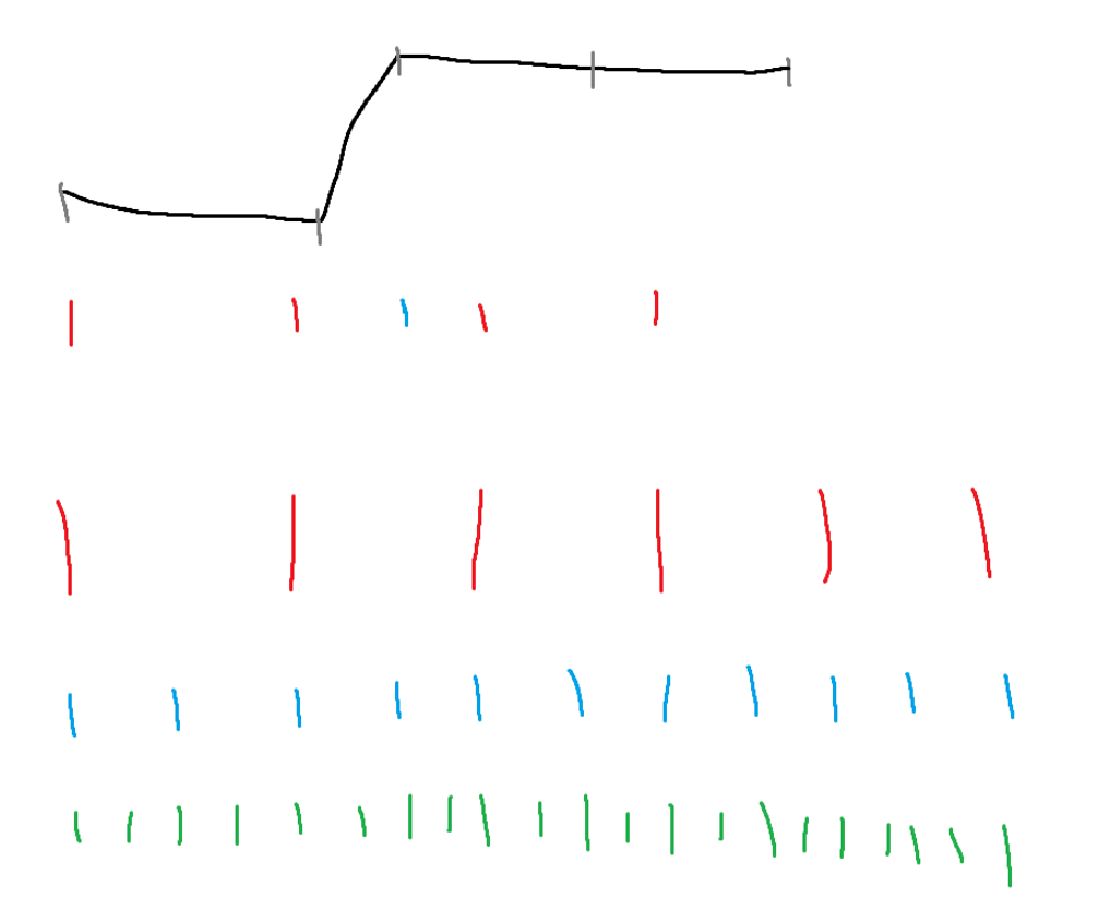
(The data representations for this method were all with respect to a given point, for example if I could ensure that the convexity defect in each hull is consistent across pairs of similar edges, I could use them as an anchor point by aligning them first, then handling scale/orientation differences after)
I then iterated any 2 edgePairs that had similar representations/sampling rates like this:
This was done by querying a bounding volume hierarchy of similarly-sampled line segments in each edge under distance and angle constraints (annulus sector):
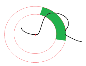
Since I was working with line segments rather than points, there is a range of values where the angle covered by a line segment from one edge may overlap with that of a line segment from another edge. In the diagram below there is a (angular?) representation of a group of line segments of various sample rates labeled query. On the left the top line is another representation of a group of line segments. I notice that the 1st subarea/lineSegment in the query was sampled at the same rate (red) as the 1st subarea in the group on the left. So to begin trying to align/match/test these 2 groups, I must first find the range of values that the 1st subarea in the query can be shifted while still having non-zero overlap with the 1st subarea in the other group. The arrows on the 2nd line on the left show the 1st query subarea being shifted max left and max right.
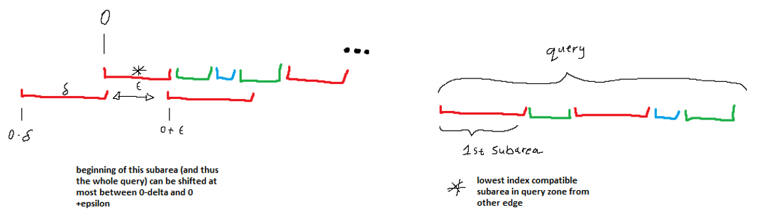
I then constrained the maximum shift of the whole query group by this value, and continued to the second query subarea and so on. If there was a range of values that the query group could be shifted while ensuring each subarea within the query had at least 1 point of overlap with a similarly-sampled subarea in the other group then I proceeded, if not then I assumed the 2 edges were incompatible and skipped them.
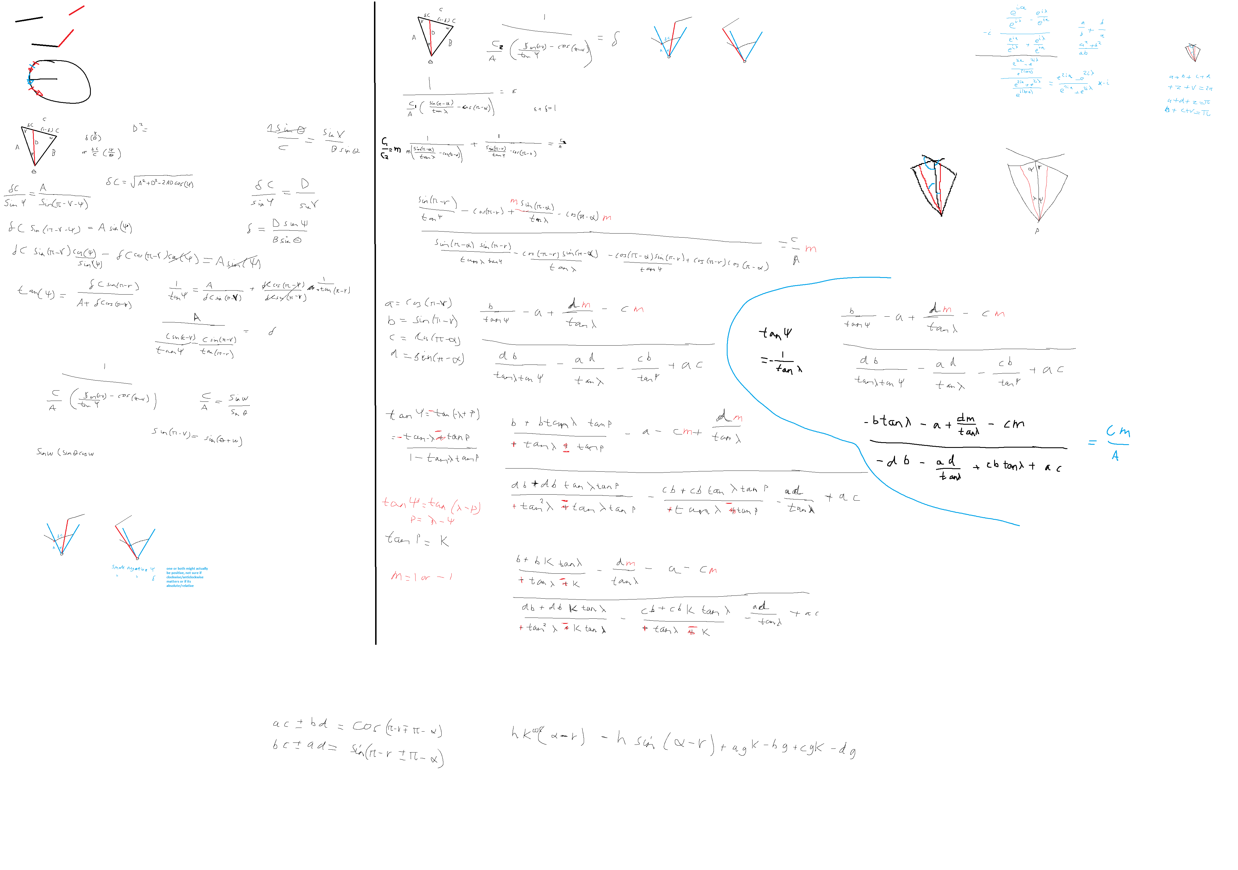
Below is a sample of some of the maths involved in calculating the maximum shift/wiggle range for 2 subareas, the code that implements this maths starts here and ends roughly 700 lines later at the end of the function.
This method wasn’t too bad but it still struggled to handle edges being split into 2 parallel planes as that added far too much ambiguity on top of the already ambiguous problem of part-to-part shape matching with scale, orientation and starting point correspondence unknowns.
I then spent some time trying to find a way to constrain degrees of freedom related to the parallel planes and that's when I noticed the relationship between the plane swapping of the edge contours and the line from the centre image point (or orthogonal plane point w.r.t. camera coords) that I described previously. Assuming/asserting that the image plane will be parallel-enough to the table plane was enough to constrain the problem to a satisfactory and reasonable level.
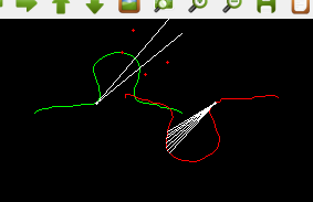
Another scrapped idea was to use the scale difference between pointPairs obtained by ray shooting and using the orientation that gave the most flat distribution of scales:
Conceptualised and partially implemented an algorithm to assemble large groups of pieces (rather than just finding the best edge pairings)
(This was cut short due to real life time constraints)The algorithm iterates assembly in a tree-like fashion rather than generic permutations as to avoid any duplicate sub-structures appearing in the group formation. Conflict resolution may be solved by treating each layout as a flow network with similarity scores being the edge weights and using a max flow algorithm (Ford–Fulkerson or Edmonds–Karp) to find the edge pairing/s that should be discarded to optimise confidence in the current puzzle layout (see max-flow min-cut theorem).
